Often locations need to be connected by a network of paths to allow for movement between them. For example:
Timber (need to improve the examples
Fire fighters
Military locations
Habitat patches
The Cost Connectivity tool creates the least-cost, optimum network of corridors connecting a series of input regions. On the resulting network, the phenomenon being modeled can move from any region to any other region using the corridors.
Prior to Cost Connectivity, networks of least cost paths were assembled by running Cost Distance/Cost Path iteratively for each set of regions and combining individual least-cost paths.
Facebook Twitter Share
The Cost Connectivity Input - The Regions
Cost Connectivity requires two input:
The regions to connect
A surface identifying the cost or preference surface the mover will encounter as they travel through each location in the landscape.
Several habitat patches suitable for bobcat (Lynx rufus) have been identified in a northern portion of Vermont, USA. In order to maintain healthy genetic diversity between these bobcat metapopulations, all habitat patches, or regions, must be connected to each other within a network of wildlife corridors. Furthermore, a network of paths would allow bobcats to recolonize a region that goes locally extinct.
The Cost Connectivity tool is designed to solve problems such as this one and other connectivity issues.
The bobcat habitat parches to connect are in green displayed over a hillshade.
Facebook Twitter Share
The Cost Connectivity Input - The Cost Surface
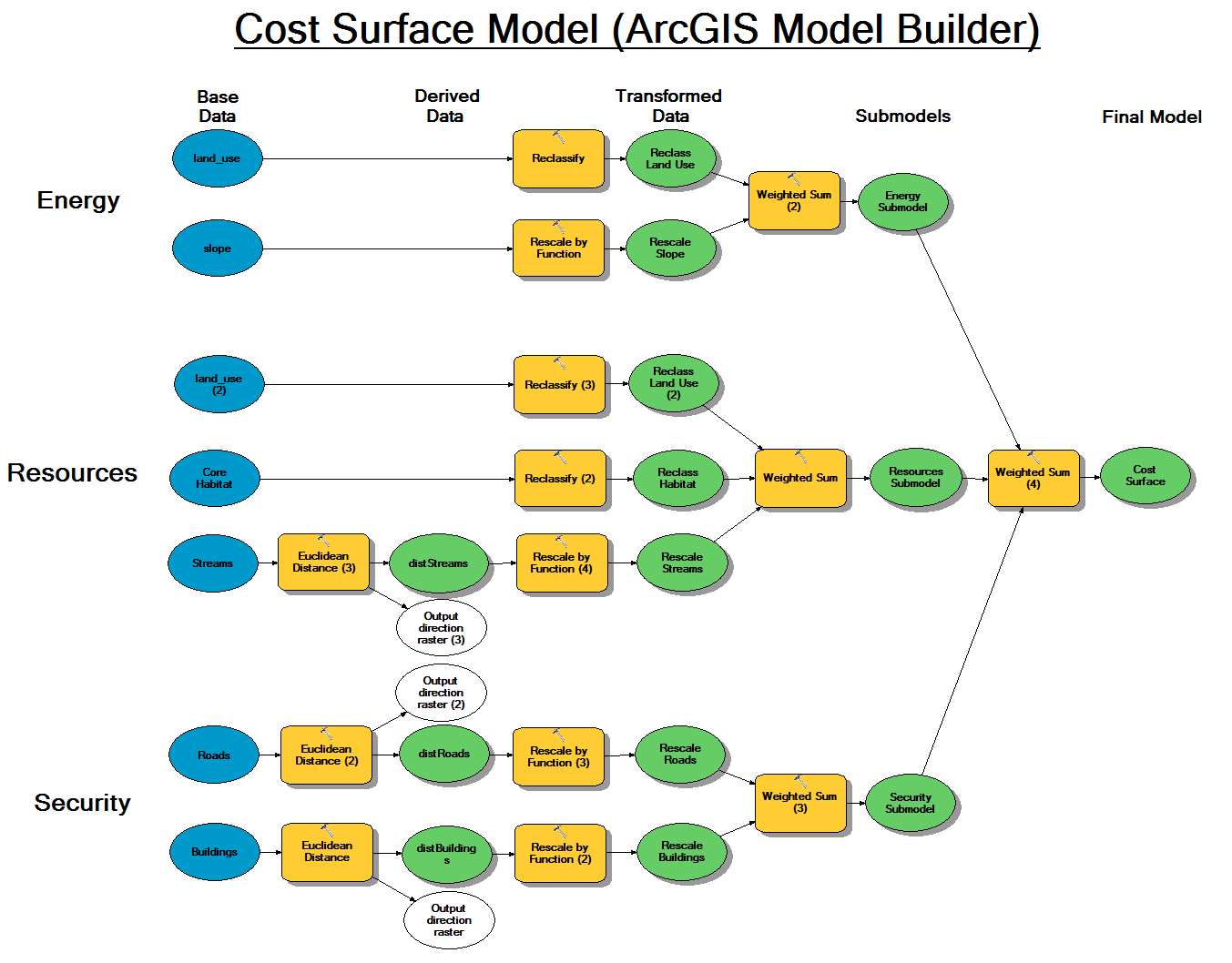
The cost surface identifies how costly it is for a phenomenon to move across the surface. Raster cells with lower cost are more preferred.
A cost raster usually combines multiple criteria, similar to suitability modeling. Contrary to a suitability model, a cost model focuses on criteria affecting movement. For more information on suitability modeling see Understanding the Suitability Modelling workflow.
Land use and slope, among other criteria, are combined to create a cost surface model for bobcats traveling through the landscape.
The cost surface is displayed in the Map. The brighter green are least costly with brighter red locations being the most costly.
Cost Connectivity utilizes the cost surface to identify least-cost paths between regions, a process detailed in the next section.
Facebook Twitter Share
Understanding How Cost Connectivity Works
The ultimate goal of Cost Connectivity is to create a network of paths between the regions so that any region can access any other region through the network.
Conceptually Cost Connectivity works as follows:
Cost Distance is run using each input regions a a unique source to determine the accumulative cost for each cell to reach each source.
Cost Allocation is run to identify which regions are the cost neighbors for each input region.
Cost paths are created between each region and its neighboring cost neighbor using the resulting cost distance and back link rasters produced in step 1. All the cost paths to their neighboring cost neighbors are combined.
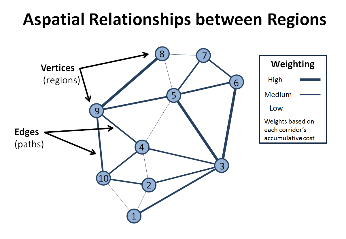
The regions and the resulting combined cost paths are converted to an aspatial graph.
The Minimum Spanning Tree is determined using graph theory to connect the regions in the most effective, (least costly) way possible.
The spatial representation of the regions and the corridors from the minimum spanning tree are output as a feature class.
Optionally, a feature class of the regions and all the corridors to the neighboring cost regions can be output.
Paths between some regions may pass through another region or multiple regions.
In the Map, six regions are connected by the optimum least-cost network of paths.
Facebook Twitter Share
Using Cost to Define Which Regions Should be Connected
To identify which regions should be connected to which region Cost Allocation, and not Euclidean Allocation, is used within the Cost Connectivity algorithm. This is because two regions can be close to one another in Euclidean distance but be far apart in cost distance.
In the Map the Cost Allocation is displayed. It is cheaper for cells of the same color to reach the region encompassed by that color. Paths will be created from each region to its neighboring cost region. In Euclidean Allocation the configuration of the resulting zones is different than the Cost Allocation configuration of zones. In many cases, even the neighbors can be different.
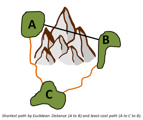
Cost Allocation is used as the basis for defining which regions should be connect since two regions (region A and region B) are clearly closer together than a third (region c). It would make sense that the two closer regions are connected by a path directly between them than one that uses the third regions as a stepping stone to get to the other.
Now suppose a mountain exists between regions A and B. Even though a path directly to region B from region A is shorter, less energy is spent traveling to region B via region C rather than traversing the mountain. In essence, the shortest path is not always the quickest, and hence why Cost Distance and Cost Allocation are utilized within Cost Connectivity.
Facebook Twitter Share
Connecting Paths Within Regions
As corridors reach a region boundary, the cost stops accumulating because cost distance calculates accumulating cost from the edge of each region. Here is how corridors connect within regions.
Recall that graph theory, which is needed to solve the minimum spanning tree, requires an aspatial representation of regions and corridors. Since there is essentially no cost to move within a region, each region automatically becomes a node in graph theory with multiple corridors (edges) connecting to it.
When the aspatial graph theory representation of the network is converted back to the original spatial configuration, corridors are extended (without additional cost) from the region boundary to a central point. This point acts as a hub where all incoming and outgoing corridors meet. It is at this point where phenomena moving along a corridor can switch to another corridor.
Facebook Twitter Share
Adding Paths to a Network
The output from Cost Connectivity may or may not be ready for further analysis depending on its use. Perhaps the addition of another, or multiple paths, to the optimum network based on the minimum spanning tree algorithm is necessary.
Specific paths can be added for specific reasons, such as escape or access routes in the case of firefighters. One additional path has been added to the minimum spanning tree connecting bobcat habitat patches to skirt a populated area.
Paths can also be added based on specific capabilities such as source characteristics or directionality. Additional paths are created using Cost Distance/Cost Path tools, and then joining the new path with the Cost Connectivity output.
Facebook Twitter Share
Removing Paths from a Network
In some cases, the overall cheapest series of corridors (minimum spanning tree) may not provide enough information. Alternatively, Cost Connectivity can generate an output of all corridors to the neighboring cost regions.
Networks can be personalized and custom-fit to scenarios by reducing the number of corridors through expert opinion or corridor statistics. Each corridor has multiple attribute fields: accumulative cost, patches connected, and corridor length.
Click on corridors to the right to see their statistics. Which ones might you remove?
Facebook Twitter Share
Care When Defining Raster Input Regions
The goal of Cost Connectivity is to connect regions, but in order to do so each region must be unique.
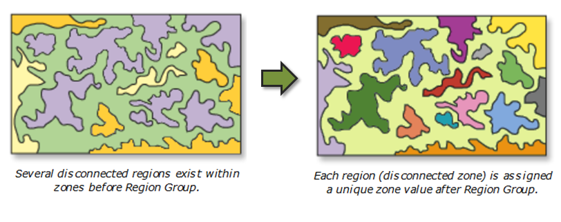
In this example, a land use raster has been simplified into forested and non-forested zones. Each cell is included in either the forested zone (green) if it has a value of 1, or the non-forested zone (beige) if it has a value of 2. At this point, even though groups of forest are visually disconnected from one another into regions, each region is not uniquely identified.
A region can be defined as a contiguous group of cells where each cell is the same value. Therefore, a disconnected zone is made up of smaller, contiguous regions. To identify each region, the Region Group tool is run. This assigns a unique value to each region, the necessary step to input a regions layer into Cost Connectivity.
Facebook Twitter Share
Using Points as Regions
Raster layers and polygon feature classes are not the only types of regions Cost Connectivity can create a network for. Points can also be used as regions.
Consider several locations of fire fighters stationed in remote areas to watch for and combat wildfires. In the case of a fire, some of these outposts may need extra manpower from the other stations to help contain the fire. Cost Connectivity can be used to identify the most optimum, least-costly network linking all firefighter groups.
Facebook Twitter Share
Analyzing Cost Connectivity with Network Analyst
Further analysis can be conducted with the output feature class of regions and corridors from Cost Connectivity by converting it into a Network Analyst network.
The Network Analyst extension is capable of performing six types of analysis:
Route
Service Area
Closest Facility
Origin-Destination Cost Matrix
Vehicle Routing
Location-Allocation
Network Analyst can help answer questions such as:
What is the quickest way to get from A to B?
Which houses are five minutes of a fires station?
What market area does a business cover?
Acknowledgements
We thank Steven Lamonde of Johnson State College and the Vermont Center for Geographic Information for their contributions.
Often locations need to be connected by a network of paths to allow for movement between them. For example:
Timber (need to improve the examples
Fire fighters
Military locations
Habitat patches
The Cost Connectivity tool creates the least-cost, optimum network of corridors connecting a series of input regions. On the resulting network, the phenomenon being modeled can move from any region to any other region using the corridors.
Prior to Cost Connectivity, networks of least cost paths were assembled by running Cost Distance/Cost Path iteratively for each set of regions and combining individual least-cost paths.
Facebook Twitter Share
Tap for details
Swipe to explore
LEARN MORE
Tap to go back
Swipe to explore
The Cost Connectivity Input - The Regions
Cost Connectivity requires two input:
The regions to connect
A surface identifying the cost or preference surface the mover will encounter as they travel through each location in the landscape.
Several habitat patches suitable for bobcat (Lynx rufus) have been identified in a northern portion of Vermont, USA. In order to maintain healthy genetic diversity between these bobcat metapopulations, all habitat patches, or regions, must be connected to each other within a network of wildlife corridors. Furthermore, a network of paths would allow bobcats to recolonize a region that goes locally extinct.
The Cost Connectivity tool is designed to solve problems such as this one and other connectivity issues.
The bobcat habitat parches to connect are in green displayed over a hillshade.
Facebook Twitter Share
Tap for details
Swipe to explore
LEARN MORE
Tap to go back
Swipe to explore
The Cost Connectivity Input - The Cost Surface
The cost surface identifies how costly it is for a phenomenon to move across the surface. Raster cells with lower cost are more preferred.
A cost raster usually combines multiple criteria, similar to suitability modeling. Contrary to a suitability model, a cost model focuses on criteria affecting movement. For more information on suitability modeling see Understanding the Suitability Modelling workflow.
Land use and slope, among other criteria, are combined to create a cost surface model for bobcats traveling through the landscape.
The cost surface is displayed in the Map. The brighter green are least costly with brighter red locations being the most costly.
Cost Connectivity utilizes the cost surface to identify least-cost paths between regions, a process detailed in the next section.
Facebook Twitter Share
Tap for details
Swipe to explore
LEARN MORE
Tap to go back
Swipe to explore
Understanding How Cost Connectivity Works
The ultimate goal of Cost Connectivity is to create a network of paths between the regions so that any region can access any other region through the network.
Conceptually Cost Connectivity works as follows:
Cost Distance is run using each input regions a a unique source to determine the accumulative cost for each cell to reach each source.
Cost Allocation is run to identify which regions are the cost neighbors for each input region.
Cost paths are created between each region and its neighboring cost neighbor using the resulting cost distance and back link rasters produced in step 1. All the cost paths to their neighboring cost neighbors are combined.
The regions and the resulting combined cost paths are converted to an aspatial graph.
The Minimum Spanning Tree is determined using graph theory to connect the regions in the most effective, (least costly) way possible.
The spatial representation of the regions and the corridors from the minimum spanning tree are output as a feature class.
Optionally, a feature class of the regions and all the corridors to the neighboring cost regions can be output.
Paths between some regions may pass through another region or multiple regions.
In the Map, six regions are connected by the optimum least-cost network of paths.
Facebook Twitter Share
Tap for details
Swipe to explore
LEARN MORE
Tap to go back
Swipe to explore
Using Cost to Define Which Regions Should be Connected
To identify which regions should be connected to which region Cost Allocation, and not Euclidean Allocation, is used within the Cost Connectivity algorithm. This is because two regions can be close to one another in Euclidean distance but be far apart in cost distance.
In the Map the Cost Allocation is displayed. It is cheaper for cells of the same color to reach the region encompassed by that color. Paths will be created from each region to its neighboring cost region. In Euclidean Allocation the configuration of the resulting zones is different than the Cost Allocation configuration of zones. In many cases, even the neighbors can be different.
Cost Allocation is used as the basis for defining which regions should be connect since two regions (region A and region B) are clearly closer together than a third (region c). It would make sense that the two closer regions are connected by a path directly between them than one that uses the third regions as a stepping stone to get to the other.
Now suppose a mountain exists between regions A and B. Even though a path directly to region B from region A is shorter, less energy is spent traveling to region B via region C rather than traversing the mountain. In essence, the shortest path is not always the quickest, and hence why Cost Distance and Cost Allocation are utilized within Cost Connectivity.
Facebook Twitter Share
Tap for details
Swipe to explore
LEARN MORE
Tap to go back
Swipe to explore
Connecting Paths Within Regions
As corridors reach a region boundary, the cost stops accumulating because cost distance calculates accumulating cost from the edge of each region. Here is how corridors connect within regions.
Recall that graph theory, which is needed to solve the minimum spanning tree, requires an aspatial representation of regions and corridors. Since there is essentially no cost to move within a region, each region automatically becomes a node in graph theory with multiple corridors (edges) connecting to it.
When the aspatial graph theory representation of the network is converted back to the original spatial configuration, corridors are extended (without additional cost) from the region boundary to a central point. This point acts as a hub where all incoming and outgoing corridors meet. It is at this point where phenomena moving along a corridor can switch to another corridor.
Facebook Twitter Share
Tap for details
Swipe to explore
LEARN MORE
Tap to go back
Swipe to explore
Adding Paths to a Network
The output from Cost Connectivity may or may not be ready for further analysis depending on its use. Perhaps the addition of another, or multiple paths, to the optimum network based on the minimum spanning tree algorithm is necessary.
Specific paths can be added for specific reasons, such as escape or access routes in the case of firefighters. One additional path has been added to the minimum spanning tree connecting bobcat habitat patches to skirt a populated area.
Paths can also be added based on specific capabilities such as source characteristics or directionality. Additional paths are created using Cost Distance/Cost Path tools, and then joining the new path with the Cost Connectivity output.
Facebook Twitter Share
Tap for details
Swipe to explore
LEARN MORE
Tap to go back
Swipe to explore
Removing Paths from a Network
In some cases, the overall cheapest series of corridors (minimum spanning tree) may not provide enough information. Alternatively, Cost Connectivity can generate an output of all corridors to the neighboring cost regions.
Networks can be personalized and custom-fit to scenarios by reducing the number of corridors through expert opinion or corridor statistics. Each corridor has multiple attribute fields: accumulative cost, patches connected, and corridor length.
Click on corridors to the right to see their statistics. Which ones might you remove?
Facebook Twitter Share
Tap for details
Swipe to explore
LEARN MORE
Tap to go back
Swipe to explore
Care When Defining Raster Input Regions
The goal of Cost Connectivity is to connect regions, but in order to do so each region must be unique.
In this example, a land use raster has been simplified into forested and non-forested zones. Each cell is included in either the forested zone (green) if it has a value of 1, or the non-forested zone (beige) if it has a value of 2. At this point, even though groups of forest are visually disconnected from one another into regions, each region is not uniquely identified.
A region can be defined as a contiguous group of cells where each cell is the same value. Therefore, a disconnected zone is made up of smaller, contiguous regions. To identify each region, the Region Group tool is run. This assigns a unique value to each region, the necessary step to input a regions layer into Cost Connectivity.
Facebook Twitter Share
Tap for details
Swipe to explore
LEARN MORE
Tap to go back
Swipe to explore
Using Points as Regions
Raster layers and polygon feature classes are not the only types of regions Cost Connectivity can create a network for. Points can also be used as regions.
Consider several locations of fire fighters stationed in remote areas to watch for and combat wildfires. In the case of a fire, some of these outposts may need extra manpower from the other stations to help contain the fire. Cost Connectivity can be used to identify the most optimum, least-costly network linking all firefighter groups.
Facebook Twitter Share
Tap for details
Swipe to explore
LEARN MORE
Tap to go back
Swipe to explore
Analyzing Cost Connectivity with Network Analyst
Further analysis can be conducted with the output feature class of regions and corridors from Cost Connectivity by converting it into a Network Analyst network.
The Network Analyst extension is capable of performing six types of analysis:
Route
Service Area
Closest Facility
Origin-Destination Cost Matrix
Vehicle Routing
Location-Allocation
Network Analyst can help answer questions such as:
What is the quickest way to get from A to B?
Which houses are five minutes of a fires station?
What market area does a business cover?
Acknowledgements
We thank Steven Lamonde of Johnson State College and the Vermont Center for Geographic Information for their contributions.