by Kevin M. Johnston Ph.D. Esri
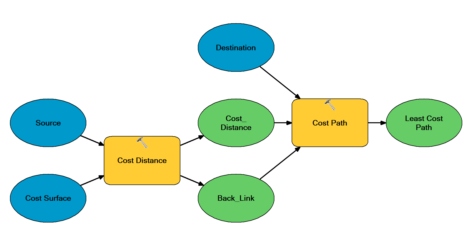
This story map will cover how to connect known source(s) with known destination(s) using the Cost Distance and Cost Path sequence of tools.
Unlike the Cost Connectivity tool which connects a series of regions with an optimum network of paths, the Cost Distance/Cost Path sequence connects defined source(s) and destination(s). However, the Cost distance/Cost Path can be used in synergy with Cost Connectivity by adding specific paths to the optimum Cost Connectivity network based on a priori information (for example, adding a second escape path for firefighters from an isolated region).
Problems addressed by using the Cost Distance/Cost Path sequence to produce a least-cost path cost include:
- Constructing road to proposed shopping center
- Conserving wildlife corridors between habitat patches
- Supplying and reinforcing military troops
- Providing movement paths for fire fighters between posts
- Locating a pipeline to connect energy fields to a refinery
- Siting electrical lines